최적의 머신러닝 모델을 위한 feature selection (특징 추출)은 매우 중요한 작업입니다. Feature의 수가 불필요하게 많게 되면 모델의 과적합이 발생하게 되고 불필요한 feature들은 모델의 예측력에 안좋은 영향을 미치게 됩니다. 직관적인 방법은 feature를 하나씩 제거하였을 때 성능에 거의 영향이 없는 feature를 중요하지 않다고 생각하여 제거하거나 도메일 지식을 활용하여 중요하지 않은 feature를 제거하거나 중요한 feature를 선택할 수 있습니다.
하지만, feature의 개수가 매우 많거나 도메인 지식이 부족한 경우에도 쉽게 feature selection 할 수 있는 방법이 있을까요? 이번 포스트에서는 대표적인 feature selection 방법 중에 하나인 BORUTA에 대해 알아보도록 하겠습니다.
BORUTA는 (폴란드 신화의 신이라고 합니다) 2010년에 공개된 R 패키지 기반의 feature selection 알고리즘으로 의사결정나무 기반의 Random forest, XGBoost 등 feature importance를 잴 수 있는 모델에 대해 동작합니다. 여러 번의 iteration을 통하여 관련이 없는 feature라고 판단할 경우 제거합니다. 간단한 예를 통해 알고리즘의 원리를 살펴보겠습니다.
Algorithm
Dummy data
공부시간, 키, 몸무게, 성적을 기록한 5개의 데이터가 있습니다. 성적이 목적 변수 (y) 이고 공부시간, 키, 몸무게 feature들이 (X) 성적에 얼마나 영향을 미치는지 알고 싶습니다.
import pandas as pd

X = pd.DataFrame({'study_hours_in_a_week': [20, 30, 45, 55, 70],
                  'height(in cms)': [182, 176, 174, 168, 181],
                  'weight(in kg)': [70, 68, 78, 61, 82]})
y = pd.Series([30, 44, 60, 68, 80], name = 'Score')

pd.concat([X,y],axis=1)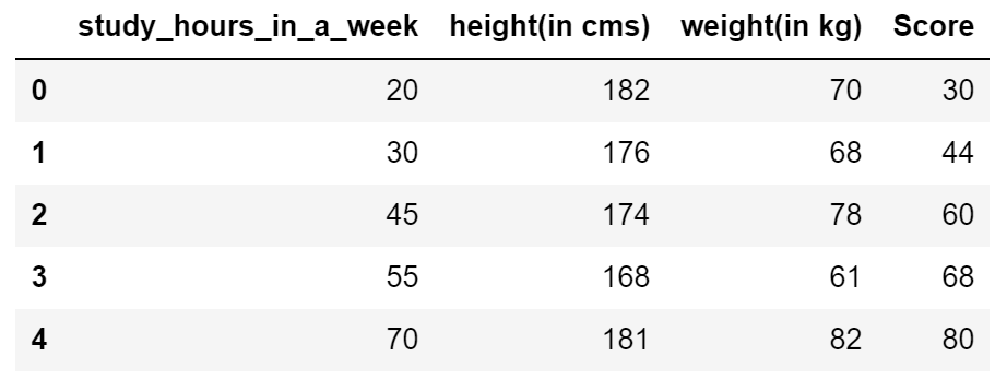
Shadow features
BORUTA의 첫 번째 스텝은 각 변수 (X)를 복사하고 복사된 변수 열을 예측 변수와 관계를 없애기 위해 랜덤하게 섞은 shadow features 를 만드는 것입니다. Shadow features 를 만들고 원래 feature 와 붙인 뒤에 feature importance를 알 수 있는 의사결정나무 기반의 Random forest, XGBoost 등의 모델로 훈련시켜 shadow features 의 feature importance 보다 작은 importance 를 가지는 본래 feature를 제거하자는 원리입니다. 먼저 shadow features 를 다음과 같이 만들고,
import numpy as np

np.random.seed(4)
X_shadow = X.apply(np.random.permutation) # Make X_shadow by randomly permuting each column of X
X_shadow.columns = ['shuffled_' + feat for feat in X.columns]

## Origin features + Shadow features
X_boruta = pd.concat([X, X_shadow], axis = 1)
X_boruta
feature importance 를 알 수 있는 모델로 (여기서는 RandomForestRegressor) 훈련시켜 shadow features의 importance 최대값보다 importance가 낮은 원래 feature를 제거합니다. 즉, 예측에 강한 영향을 미치고 있는 feature라면 랜덤화된 shadow features의 importance보다는 높을 것이기 때문에 랜덤 feature의 importance보다 importance가 낮은 원래의 feature들은 중요하지 않을 것이란 얘기이죠.
sklearn.ensemble의 RandomForestRegressor 모델로 데이터를 훈련시킨 이후에 feature_importance_ 속성을 이용하여 모든 feature의 importance를 다음과 같이 뽑아낼 수 있습니다.
from sklearn.ensemble import RandomForestRegressor

mdl = RandomForestRegressor(max_depth=5)
mdl.fit(X_boruta, y)

## Store feature importances
feature_imp_X = mdl.feature_importances_
feature_imp_shuffled = mdl.feature_importances_[len(X.columns):]

## Round off feature importances for original and shuffled features to 2 decimal places
feature_imp_shuffled = [round(i*100,2) for i in feature_imp_shuffled]
feature_imp_X = [round(i*100,2) for i in feature_imp_X]
print('Threshold for feature importance:',max(feature_imp_shuffled))
for i in range(len(X_boruta.columns)):
    print(X_boruta.columns[i]+': '+str(mdl.feature_importances_[i]))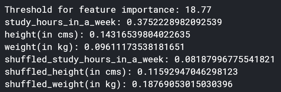
결과를 보면 shadow features의 최대 importance인 18.77보다 높은 feature는 공부시간 밖에 없고 키와 몸무게는 이보다 작으므로 제거해야 될 것으로 보입니다. 하지만 shadow features를 생성할 때 랜덤하게 변수 값을 섞었기 때문에 이를 단 한번의 결과로만 판단하기에는 무리가 있을 수 있습니다. 변수 값을 랜덤하게 생성할 때 단순히 운이 좋았을 경우도 있었을 테니까요. 이를 방지하기 위해 여러 번 수행해보도록 하겠습니다.
Iterative process
위 과정을 30번에 걸쳐 수행해보겠습니다. 즉, shadow features를 30번에 걸쳐 각각 랜덤하게 생성하고 매 수행에서 원래 feature인 공부시간, 키, 몸무게가 shadow feature importance 의 최대값인 임계치보다 높은 경우의 수를 세보겠습니다.
## Initialize hits list to count instances where the feature had importance > threhsold
hits = np.zeros((len(X.columns)))

## Perform 30 trials
for i in range(30):
   ## Create X_shuffle
   np.random.seed(i)
   X_shuffle = X.apply(np.random.permutation)
   X_boruta = pd.concat([X, X_shuffle], axis = 1)
   ## Fit random forest
   mdl = RandomForestRegressor(max_depth = 5)
   mdl.fit(X_boruta, y)
   ## Store feature importance
   feature_imp_X = mdl.feature_importances_[:len(X.columns)]
   feature_imp_shuffled = mdl.feature_importances_[len(X.columns):]
   ## Compute hits for this trial and add to counter
   hits += (feature_imp_X > feature_imp_shuffled.max())
print('Hits for every feature')
for i in range(len(X.columns)):
    print(X.columns[i],':',hits[i])
30번의 시도에서 공부시간은 24번 이상 임계치를 넘었고 키와 몸무게는 과반을 넘지 못했습니다. 특히 몸무게는 1번만 임계치가 넘었습니다. 하지만 세 개의 feature들 모두 최소 한 번 이상은 중요한 feature가 되었으므로 숫자가 적다고 무작정 제거하는 것이 아닌 통계적인 검정을 도입하여 해석하여야 합니다.
Statistical analysis
아무런 배경지식이 없을 때 50% 확률로 feature가 버려질지/존재할지 결정합니다. 즉, 통계 검정을 위한 귀무가설로는 매 순간마다 feature가 50% 확률로 중요하거나/중요하지 않거나가 결정된다는 것이죠. 따라서 귀무가설이 참으로 전제될 때의 분포로는 이항분포 (binomial)가 되며 이를 매 시도마다 확률을 그려보면 다음과 같은 정규분포 형태를 띄게 됩니다.
import scipy as sp
trials = 30
pmf = [sp.stats.binom.pmf(x, trials, .5) for x in range(1,trials + 1)]
import matplotlib.pyplot as plt
plt.xticks(np.arange(0, 31, 1))
plt.plot(range(1,6),pmf[:5],'-ro')
plt.plot(range(6,25),pmf[5:24],'-bo')
plt.plot(range(25,31),pmf[24:30],'-go')
plt.fill_between(range(1,6),pmf[:5] , color='red')
plt.fill_between(range(6,25),pmf[5:24] , color='blue')
plt.fill_between(range(25,31),pmf[24:30] , color='green')
plt.title('Plot for binomial distribution of features')
plt.xlabel('Instance count when features were important')
plt.ylabel('Binomial distribution values')
labels = ['Discard','Might be important','Keep']
plt.legend(labels,loc='upper right')
위 그림으로 봤을 때 무게 feature처럼 1번 임계치를 넘은 경우에는 통계적으로 제거하는 것이 합당해 보입니다. 또한 공부시간은 통계적으로 무조건 가지고 가야 하는 feature라 볼 수 있고 키 feature는 애매하지만 굳이 제거할 필요가 없어 보입니다.
요약
BORUTA 알고리즘을 정리하자면,
1) 모든 변수들을 복사합니다.
2) 복사한 변수 (tabular 데이터에서의 column)를 타겟에 uncorrelated 하게 만들기 위해 랜덤하게 섞습니다. (permute)
3) 원래 features와 1,2 과정을 거친 shadow features를 합칩니다. (concat)
4) Feature importance를 잴 수 있는 의사결정나무 기반의 Random forest나 XGBoost 등의 모델을 활용하여 학습합니다.
5) 학습 결과 나온 feature importance를 기반으로 shadow features의 가장 큰 feature importance를 임계치로 잡아 이보다 작은 importance를 가진 feature를 중요하지 않다고 분류합니다.
6) 1-5의 과정을 반복하여 통계적으로 유의미한 결과를 얻을 수 있도록 합니다.
다음 포스트
[Machine Learning/Data Analysis] - Feature Selection - BORUTA (2)
'Machine Learning Models > Classic' 카테고리의 다른 글
| Feature Selection - Random Forest (2) (0) | 2021.04.16 |
|---|---|
| Feature Selection - Random Forest (1) (0) | 2021.04.16 |
| Feature Selection - Recursive Feature Elimination (0) | 2021.04.09 |
| Feature Selection - Permutation Feature Importance (0) | 2021.04.09 |
| Feature Selection - BORUTA (2) (0) | 2021.04.08 |


